Eradiate Summer 2024 Dev Log

We are back with a new update format! The Dev Log series, kicked off by this post, will provide regular technical updates on our releases: What is new or changed, why we introduced some features and how to use them. In this edition, we will talk about our two latest releases, v0.27.x and v0.28.x, delivered respectively in June and August 2024. Both releases brought major performance improvements at different levels of the Eradiate stack, and we are going to see what changed.

We will discuss three major changes or improvements we made to Eradiate in those releases:

1. We introduced new infrastructure to manage molecular absorption data to overcome the limitations of the bare xarray containers we had been using so far. This resulted in a ×1.3 speed-up in typical workflows.
2. We introduced an analytical medium sampling method that addresses performance issues with plane-parallel geometries and provides speed-up up to ×150 in hyperspectral workflows.
3. We added the report of the variance of the Monte Carlo estimator in our post-processed results.

Pre-processing performance: Molecular absorption database infrastructure #

When we started working on molecular absorption simulation, we designed a database format from scratch that would provide flexibility and ease of use, while remaining compact in terms of storage. Our CKD absorption coefficient data were indexed in a lookup table that takes as parameters the central wavelength of the CKD bin, the g spectral coordinate, local pressure and temperature, and molecular species concentration.

A fundamental issue we faced since the start was that, while this type of indexing is easy to package in a NetCDF-like format (i.e. labelled n-D arrays), it is usually internally represented using dense data structures. This, in particular, means that all chemical species present in the part of the spectrum covered by the dataset will have a dimension, even if it is not radiatively active. The large number of species that are radiatively active in, at least, a part of the reflective spectral domain covered by Eradiate, makes this a major issue: a single-file database would grow in size exponentially depending on the number of species, mostly containing useless data.

We addressed this issue by splitting the database into multiple files covering a narrow spectral region, each having its own chemical species list. This resulted in a much more compact storage, as the molecules that are not active in the particular spectral interval covered by a file are not represented at all.

The next issue we ran into was data access. In order to look up these data, we need to know basic information about the dimensions and coordinates present in each file. This information was initially acquired upon dataset initialization by loading all database files and scanning their content. This, however, resulted in a potentially large memory footprint and load overhead. We added the option to restrict database loading to a small subset of the spectrum to reduce loading time, which complicated the interface. This architectural issue became critical with hyperspectral computations which would require to load and process the entire spectrum.

We solved this in v0.27.0 by introducing a molecular absorption coefficient database interface, implemented by the AbsorptionDatabase class and its subclasses. They load a molecular absorption database index which is used to perform fast queries in a multi-file database with ragged dimensions and coordinates. While the database handler can generate the index if requested by scanning all the files it references, it can also cache it and load the cache file, which cuts off loading time to a few milliseconds, almost independently of the size of the spectral database. Queries are also very fast, since each spectral interval is mapped to the relevant file by the index. Finally, the interface is simplified: the user no longer has the option or the need to restrict database loading to a specified spectral interval. Our benchmarks showed that on a typical hyperspectral workload, this improvement cut database loading time from almost a minute to a few milliseconds, and improved computational performance with an estimated speed-up of ×1.3.

Processing performance: Analytic medium sampling and transmittance estimator #

So far, Eradiate has been using a null-collision based volumetric path tracing algorithm shipped by the Mitsuba rendering system our radiometric kernel is based on. This algorithm is extremely versatile and can accommodate any form of volume data, including meshless or procedural data sources. This, however, requires providing everywhere in the scene a majorant of the extinction coefficient, which is used to perform rejection sampling for both distance sampling (picking a distance from one point in the random walk in the participating medium to the next) and transmission estimation (computing the transmittance between two points in the medium). At this date, the algorithm uses a global majorant for the entire scene.

Typical Eradiate use cases are extremely penalized by this: the extinction coefficient is a strictly decreasing function of altitude, meaning that a global majorant to the extinction coefficient is extremely loose in the higher parts of the atmosphere and leads to an overwhelming majority of null collisions—in practice increasing the computational cost in prohibitive ways.

We addressed this issue in v0.28.0 for the plane-parallel case by switching to an analytical distance sampling and transmittance estimation method. Compared to the stock volumetric path tracer, our method is much less sensitive to the magnitude of the extinction coefficient, which results in almost constant performance regardless of extinction coefficient values. Additionally, this method produces a zero-variance transmittance estimate, which results in reduced noise in many cases. Eradiate activates this method automatically when it detects a plane-parallel atmosphere.

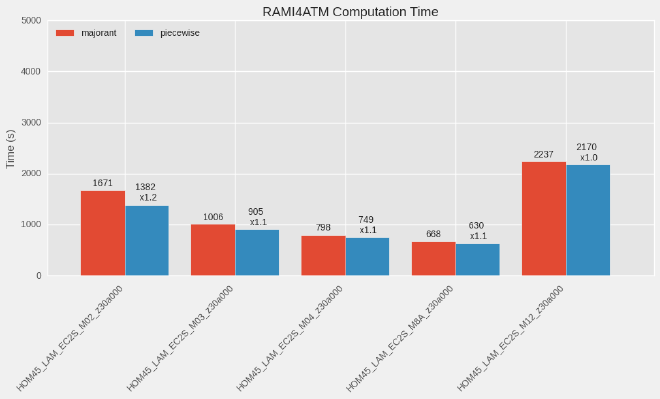
We ran benchmarks to quantify the impact of switching to this new medium sampling method. Our first benchmark uses a scene derived from the RAMI4ATM test case series, with a homogeneous discrete canopy at the surface, and a relatively low aerosol optical thickness (0.2). In this example, speed-up is between 5% and 20%. RAMI4ATM targets bands aligned with atmospheric windows where the atmosphere is almost transparent (omitting aerosols), leading to a low amount of volume interaction. Consequently, those simulations are dominated by surface interactions and the impact of improved atmospheric sampling is limited.

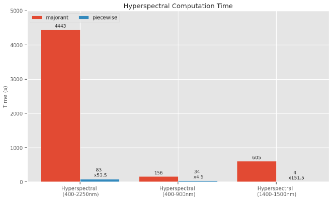
Our other benchmark is a hyperspectral computation on the [400, 2250] nm spectral interval with the default, constant-wavenumber molecular absorption database monotropa, with a light layer of aerosols (AOT 0.2). In this setup, switching to the analytical sampling method results in a speed-up between ×4.5 in the visible part of the spectrum, to ×151 in an almost opaque spectral region [1400, 1500] nm, leading to a global ×53 speed-up.

Monitoring performance: Variance report #

This is a long-awaited feature: we can now report variance for the main radiometric variable (typically radiance). We achieve this by computing the second moment of the Monte Carlo estimator, then post-processing this value together with the mean value to derive variance. This feature, introduced in Eradiate v0.28.0, is activated by setting the moment parameter of any integrator to True.

The resulting dataset is then added a variable with the _var suffix (e.g. radiance_var) with the same coordinates as the parent variable. This variance is expected to decrease quadratically with the sample count, i.e. in \(\mathrm{O} (1 / N^2) \).

Variance is of interest when is comes to estimating the uncertainty associated with simulation results. One can derive from it a standard deviation, which can then be turned into an uncertainty.

What’s next? #

We left a few points open:

• The absorption database layout can be optimized to reduce the number of files and simplify data handling. This is foreseen in the future and should make data distribution much simpler.
• We leave for later the task of finding a method to improve sampling efficiency in spherical-shell geometries. This is a significant challenge due to the added complexity of working with a spherical geometry and coordinate system, and a more generic solution that also accommodates 3D atmospheric heterogeneities might be preferable.

That being said, the features introduced in this post provide a significant performance boost for 1D hyperspectral use cases, which is a strong focus for us this year. If you have feedback about this, please do not hesitate to reach out to us.